Example 101 “Getting Started”

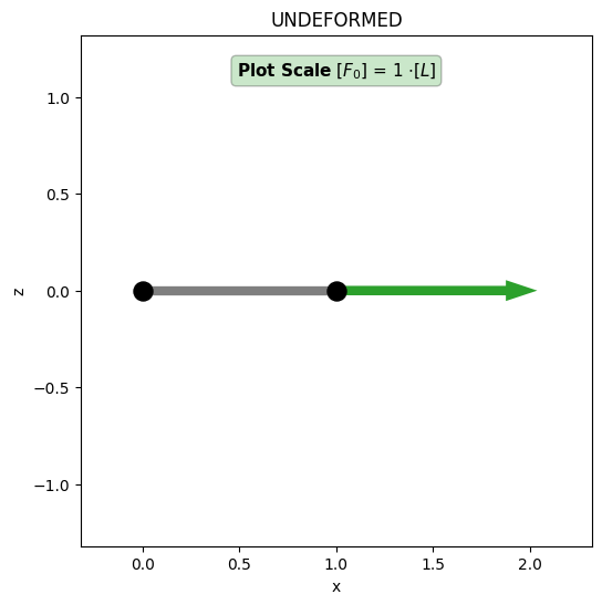
The following basic example is written in interactive mode to show how trusspy works. All model parameters except allowed incremental quantities are assumed with default values to enable a clean tutorial for the model creation process. We will consider a model with two nodes and one truss. Although this configuration does not include any geometric nonlinear effects it is the most basic example to start with. The left end of the truss (Node 1) is fixed whereas the right end displacement is free in direction x (Node 2). An external force acts on the right end of the truss in direction x. To sum up, this model contains two nodes, one element and one degree of freedom (DOF).

First we import trusspy with it’s own namespace and create a Model object. (Ensure to have trusspy installed.)

!pip install trusspy

import trusspy as tp

M = tp.Model()

Now we create Nodes with coordinate triples and Elements with a list of node connectivities and both material and geometric properties. Both Nodes and Elements are identified with their label.

# create nodes
with M.Nodes as MN:
    MN.add_node(1, (0, 0, 0))
    MN.add_node(2, (1, 0, 0))

E = 1
A = 1

# create element
with M.Elements as ME:
    ME.add_element(1, conn=[1, 2], material_properties=[E], geometric_properties=[A])
    # ME.assign_material("all", [E]) # set one value for all elements
    # ME.assign_geometry("all", [A]) # set one value for all elements

Mechanical boundary conditions must be supplied for all nodes which contain locked DOF’s: 0 = inactive (locked) and 1 = active (free). The same applies to external forces - no External Force object has to be added to the Model if all components of a node are zero.

# create displacement (U) boundary conditions
with M.Boundaries as MB:
    MB.add_bound_U(1, (0, 0, 0))
    MB.add_bound_U(2, (1, 0, 0))

# create external forces
with M.ExtForces as MF:
    MF.add_force(2, (1, 0, 0))

We have to specify some important Settings Parameters concerning the trusspy path-tracing algorithm:

M.Settings.dlpf = 0.02  # maximum allowed incremental load-proportionality-factor
M.Settings.du = 0.02  # maximum allowed incremental displacement component
M.Settings.incs = 50  # maximum number of increments

We are now able to build the model and run the job. The nodal ordering of Nodes, Boundaries and Forces inside the corresponding add function doesn’t matter. TrussPy will sort all nodal quantities by their node labels in the build method.

M.build()
fig, ax = M.plot_model()

# Model Summary
Analysis Dimension      "ndim": 3
Number of Nodes       "nnodes": 2
Number of Elements    "nelems": 1
 
System DOF              "ndof": 6
active DOF             "ndof1": 1
locked DOF             "ndof2": 5
 
active DOF          "nproDOF1": [3]
fixed  DOF          "nproDOF0": [0 1 2 4 5]

M.run()

When the job has finished we may post-process the deformed model and plot the force-displacement curve at Node 2.

fig, ax = M.plot_model(
    view="xz",
    contour="force",
    inc=-1,
)

The deformed model with the current External Force vector acting on Node 2.

fig, ax = M.plot_history(nodes=[2, 2], X="Displacement X", Y="Force X")

The load-displacement curve for all increments at Node 2.

It could also be helpful to show the animated deformation process within a simple GIF file (options should be self-explaining). The resulting movie is saved to figures/gif/movie.gif whereas all deformed states are saved as figures/png/fig_###.png

M.plot_movie(
    view="xz",
    contour="force",
    lim_scale=(-0.5, 3.5, -2, 2),
    force_scale=1.0,
    cbar_limits=[-1, 1],
)

Important Note: A LOT of assumptions are made to run this model without specifying barely any parameter. Most important ones are incremental displacement values, incremental LPF value and the amount of increments to be solved. These critical parameters are responsible if the model solution will converge or not!